Graph Diffusion Convolution

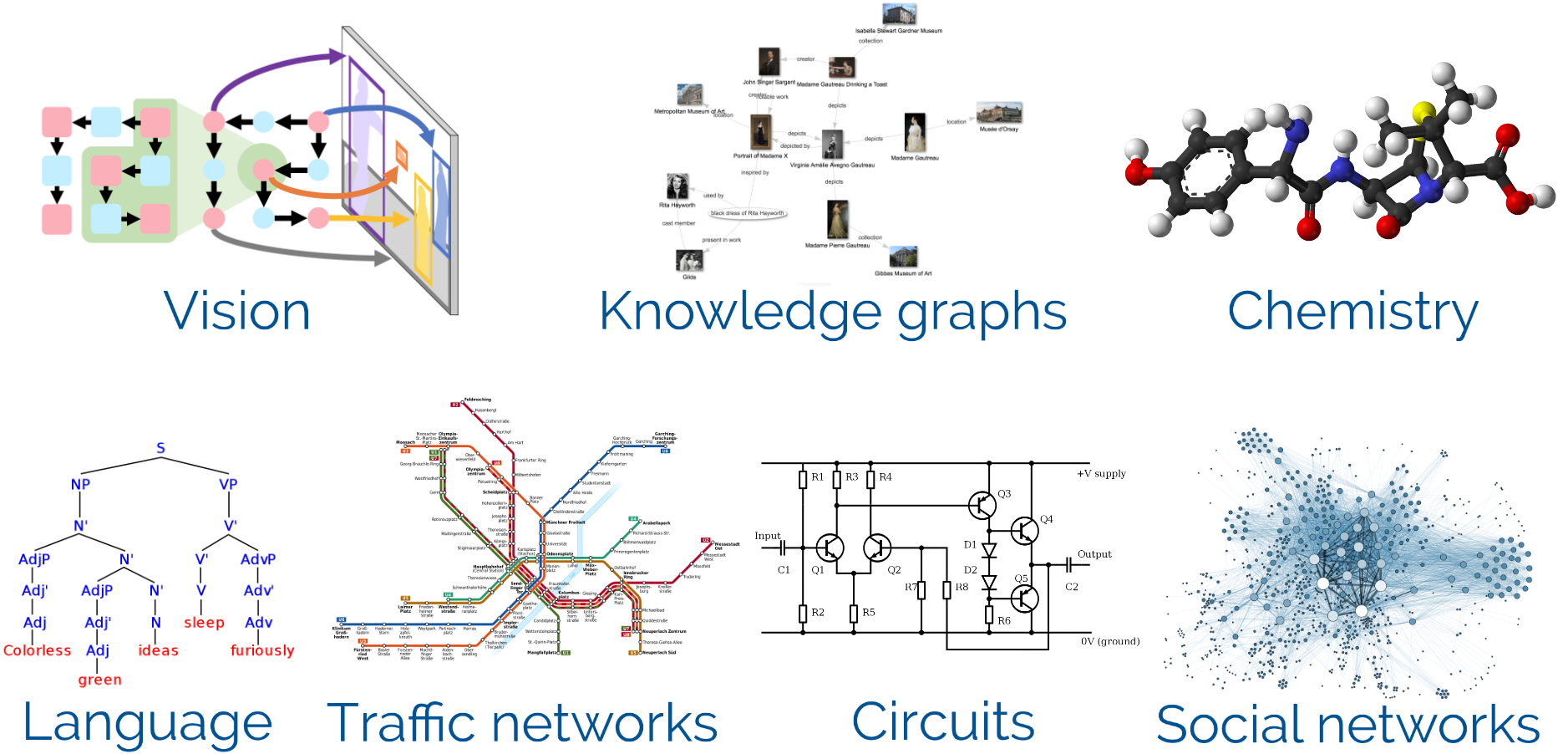
In almost every field of science and industry you will find applications that are well described by graphs (a.k.a. networks). The list is almost endless: There are scene graphs in computer vision, knowledge graphs in search engines, parse trees for natural language, syntax trees and control flow graphs for code, molecular graphs, traffic networks, social networks, family trees, electrical circuits, and so many more.

Some examples of graphs. [Wikimedia Commons, Stanford Vision Lab]

While graphs are indeed a good description for this data, many of these data structures are actually artificially created and the underlying ground truth is more complex than what is captured by the graph. For example, molecules can be described by a graph of atoms and bonds but the underlying interactions are far more complex. A more accurate description would be a point cloud of atoms or even a continuous density function for every electron.

So one of the main questions when dealing with graphical data is how to incorporate this rich underlying complexity while only being supplied with a simple graph. Our group has recently developed one way of leveraging this complexity: Graph diffusion convolution (GDC). This method can be used for improving any graph-based algorithm and is especially aimed at graph neural networks (GNNs).

GNNs have recently demonstrated great performance on a wide variety of tasks and have consequently seen a huge rise in popularity among researchers. In this blog post I want to first provide a short introduction to GNNs and then show how you can leverage GDC to enhance these models.

What are Graph Neural Networks?

In each layer the node $\nu$ receives messages from all neighboring nodes $w$ and updates its embedding based on these messages. The node embeddings before the first layer are usually obtained from some given node features. In citation graphs, where papers are connected by their citations, these features are typically a bag-of-words vector of each paper’s abstract.

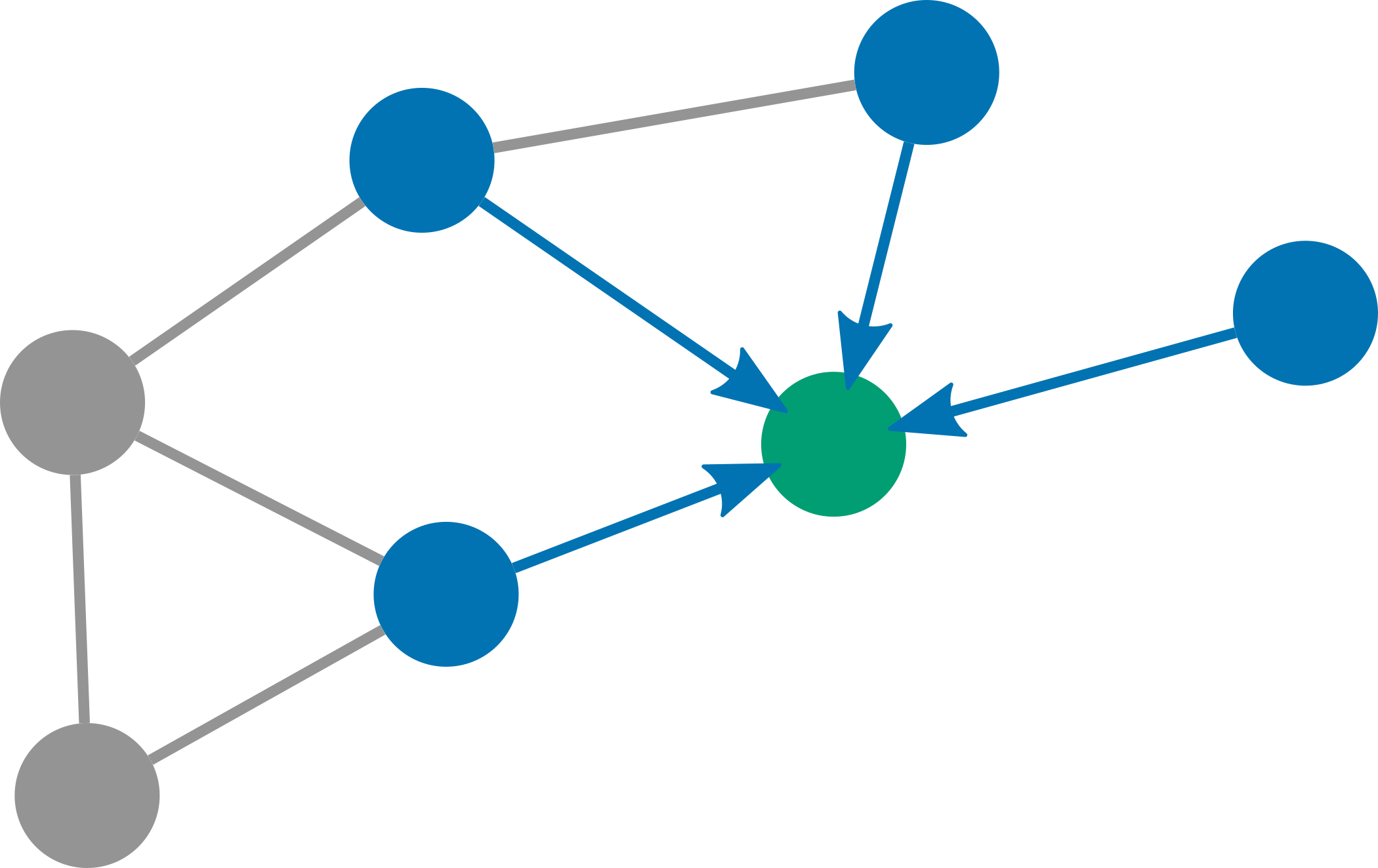
The idea behind graph neural networks (GNNs) is rather simple: Instead of making predictions for each node individually we pass messages between neighboring nodes after each layer of the neural network. This is why one popular framework for GNNs is aptly called Message Passing Neural Networks (MPNNs). MPNNs are defined by the following two equations:

$$m_{v}^{(t+1)}=\sum_{w \in N(v)} f_{\text {message}}^{(t+1)}\left(h_{v}^{(t)}, h_{w}^{(t)}, e_{v w}\right),\\ h_{v}^{(t+1)}=f_{\text {update}}^t\left(h_{v}^{(t)}, m_{v}^{(t+1)}\right)$$

where $h_{v}$ is a node embedding, $e_{v w}$ an edge embedding, $m_{v}$ an incoming message, and $\quad N_{v}$ denotes the neighbors of $v$. In the first equation all incoming messages are aggregated, with each message being transformed by a function $f_{\text {message}}$, which is usually implemented as a neural network.

The node embeddings are then updated based on the aggregated messages via $f_{\text{update}}$, which is also commonly implemented as a neural network. As you can see, in each layer of a GNN a single message is sent and aggregated between neighbors. Each layer learns independent weights via backpropagation, i.e. $f_{\text{message}}$ and $f_{\text{update}}$ are different for each layer. The arguably most simple GNN is the Graph Convolutional Network (GCN), which can be thought of as the analogue of a CNN on a graph. Other popular GNNs are PPNP, GAT, SchNet, ChebNet, and GIN.

The above MPNN equations are limited in several ways. Most importantly, we are only using each node’s direct neighbors and give all of them equal weight. However, as we discussed earlier the underlying ground truth behind the graph is usually more complex and the graph only captures part of this information. This is why graph analysis in other domains has long overcome this limitation and moved to more expressive neighborhoods (since around 1900, in fact). Can we also do better than just using the direct neighbors?

Going beyond direct neighbors: Graph diffusion convolution

GNNs and most other graph-based models interpret edges as purely binary, i.e. they are either present or they are not. However, real relationships are far more complex than this. For example, in a social network you might have some good friends with whom you are tightly connected and many acquaintances whom you have only met once.

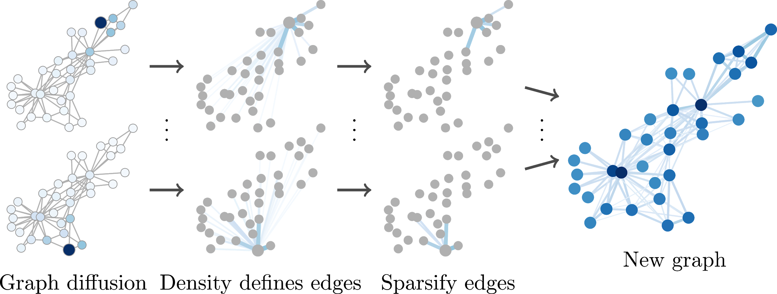
To improve the predictions of our model we can try to reconstruct these continuous relationships via graph diffusion. Intuitively, in graph diffusion we start by putting all attention onto the node of consideration. We then continuously pass some of this attention to the node’s neighbors, diffusing the attention away from the starting node. After some time we stop and the attention distribution at that point defines the edges from the starting node to each other node. By doing this for every node we obtain a matrix that defines a new, continuously weighted graph. More precisely, graph diffusion is defined by

$$S=\sum_{k=0}^{\infty} \theta_{k} T^{k}$$

where $\theta_{k}$ are coefficients and $T$ denotes the transition matrix, defined e.g. by $A D^{-1},$ with the adjacency matrix $A$ and the diagonal degree matrix $D$ with $d_{i i}=\sum_{j} a_{i j}$.

These coefficients are predefined by the specific diffusion variant we choose, e.g. personalized PageRank (PPR) or the heat kernel. Unfortunately, the obtained $S$ is dense, i.e. in this matrix every node is connected to every other node. However, we can simply sparsify this matrix by ignoring small values, e.g. by setting all entries below some threshold $\varepsilon$ to $0 .$ This way we obtain a new sparse graph defined by the weighted adjacency matrix $\tilde{S}$ and use this graph instead of the original one. There are even fast methods for directly obtaining the sparse $\tilde{S}$ without constructing a dense matrix first.

Graph diffusion convolution (GDC): We first perform diffusion on the original graph, starting from some node $\nu$. The density after diffusion defines the edges to the starting node $\nu$. We then remove all edges with small weights. By doing this once for each node we obtain a new sparse, weighted graph $S$.

Hence, GDC is a preprocessing step that can be applied to any graph and used with any graph-based algorithm. We conducted extensive experiments (more than 100,000 training runs) to show that GDC consistently improves prediction accuracy across a wide variety of models and datasets. Still, keep in mind that GDC essentially leverages the homophily found in most graphs. Homophily is the property that neighboring nodes tend to be similar, i.e. birds of a feather flock together. It is therefore not applicable to every dataset and model.

Why does this work?

Up to this point we have only given an intuitive explanation for GDC. But why does it really work? To answer this question we must dive a little into graph spectral theory.

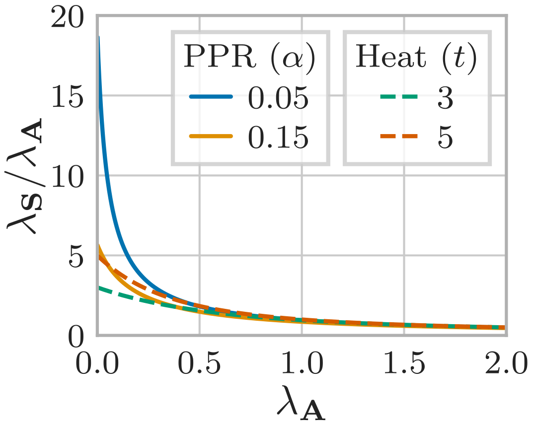
In graph spectral theory we analyze the spectrum of a graph, i.e. the eigenvalues of the graph’s Laplacian $L=D-A$, with the adjacency matrix $A$ and the diagonal degree matrix $D$. The interesting thing about these eigenvalues is that low values correspond to eigenvectors that define tightly connected, large communities, while high values correspond to small-scale structure and oscillations, similar to the small and large frequencies in a normal signal. This is exactly what spectral clustering takes advantage of.

When we look into how these eigenvalues change when applying GDC, we find that GDC typically acts as a low-pass filter. In other words, GDC amplifies large, well-connected communities and suppresses the signals associated with small-scale structure. This directly explains why GDC can help with tasks like node classification or clustering: It amplifies the signal associated with the most dominant structures in the graph, i.e. (hopefully) the few large classes or clusters we are interested in.

GDC acts as a low-pass filter on the graph signal. The eigenvectors associated with small eigenvalues correspond to large, tightly connected communities. GDC therefore amplifies the signals that are most relevant for many graph-based tasks.

Further Information

If you want to get started with graph neural networks I recommend having a look at PyTorch Geometric, which implements many different GNNs and building blocks to create the perfect model for your purposes. I have already implemented a nice version of GDC in this library.

If you want to have a closer look at GDC I recommend checking out our paper and our reference implementation, where you will find a notebook that lets you reproduce our paper’s experimental results.

@inproceedings{klicpera_diffusion_2019,
    title = {Diffusion Improves Graph Learning},
    author = {Klicpera, Johannes and Wei{\ss}enberger, Stefan and G{\"u}nnemann, Stephan},
    booktitle = {Conference on Neural Information Processing Systems (NeurIPS)},
    year = {2019}
}