Is this my body? (Part I)

We wake up every morning and we look in the mirror and… yes, that reflexion is you. How do we know it? How do we know where our body parts are in space or that we produced that effect in the environment? Surprisingly, our joint sensors proprioception (e.g. muscle spindles) are nothing but imprecise and we do not even have exact models of the body and the world. Despite that, we are able to have robust control of our body for general purpose tasks and, at the same time, we are flexible enough to adequate all the changes that happen in our body during life. We might think that we achieved general intelligence due to body imprecision. In fact, adaptation and learning will be two of the core processes that allow us to interact in an uncertain world.

On the one hand, we know that humans create a sensorimotor mapping in the brain by learning the relation between different sensations (cross/multimodal learning). On the other hand, experiments have shown us that body perception is rather flexible with an instantaneous strong (bottom-up) component. For instance, in less than one minute we can make you think that your limb is a plastic hand in a different location or transfer as yours the body of a friend (body transfer illusion) just by visuotactile stimulation. This effect was first discovered by means of the rubber-hand illusion and presents body perception as a very flexible and instantaneous process. This is a commonly observed effect in virtual reality where your body is different but it is rapidly integrated.

The challenge: Robots, conversely, usually have a fixed body and precise sensors and models. Then, why do they still perform poorly with their body in real-world uncertain situations?

Perception as inference in the brain

Visual illusions are a great source of information to understand how perception works in the brain. In the following figure, Dallenbach’s illusion is presented. If you have never seen the solution, it will be hard to see what is in the picture. However, after observing the solution it will be easy to recognize it.

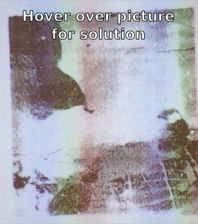
But the crucial and astonishing consequence is that no matter what you do you afterward, you will always see the same concept in the picture. It is like a seed has been placed in your brain and stays forever. According to the medical doctor and physicist Hermann von Helmholtz, visual perception is an unconscious mechanism that infers the world. In my approach, the brain has generative models that complete or reconstruct the world from partial information. In Dallenbach’s illusion example, the prior information helps to reconstruct the animal in the image.

Assuming that the brain is perceiving the world in this manner, then body perception should have a similar process behind.

The free-energy principle

The free-energy principle (FEP), proposed by Karl Friston, presents the brain as a Markov blanket that has only access to the world through the body senses. Conceptually, body perception and action are a result of surprise minimization. Mathematically, it can be classified as a variational inference method as it uses the minimization of the variational free energy bound for tractability. This bound has been largely investigated in the machine learning community and it is a concept that was originated in the field of physics.

Notation tip: Be aware that I will use notation and terminology that sometimes confuses if you are familiar with variational inference. In this post observations are $s$ and the hidden variables are $x$.

Let us imagine that we want to infer our body posture $x$ (latent state) from the information provided by all body sensors $s$. Using the Bayes rule we obtain:

$$p(x | s)=\frac{p(s | x) p(x)}{p(s)}$$

That is the likelihood of observing that specific sensor information given my posture multiplied by my prior knowledge of my posture, divided by the total probability. In order to compute the denominator, we have to integrate over all possible states of the body. This is in practice intractable for continuous spaces.

Fortunately for us, we can do a workaround by tracking the real distribution $p(x|s)$ with a reference distribution $q(x)$ with a known tractable form. Thus, our goal is to approximate $q$ to the real world distribution $p$. We can minimize the KL-divergence between the true posterior and our reference distribution, as we know that when the divergence is 0 both distributions are the same. But instead of directly minimizing it, we are going to use a lower bound called negative variational free energy $F$ or evidence lower bound (ELBO).

$$D_{K L}(q(x) \| p(x | s))=F+\ln p(s)$$

where $\ln p(s)$ is the log-evidence of the model or surprise (in the free energy principle terminology). Note that the second term does not depend on the reference distribution so we can directly optimize $F$. (We leave the derivation of the negative variational free energy bound for another post.)

The negative variational free energy is composed of two expectations:

$$F=-\int q(x) \ln p(s, x) d x+\int q(x) \ln q(x) d x$$

We can simplify $F$ further by means of the Laplace approximation. We define our reference function as a tractable family of factorized Gaussian functions. This is sometimes referred to as the Laplace encoded energy $F \approx L$. Under this assumption, we can track the reference distribution by its mean $\mu$. Thus we arrive at our final definition of the variational Laplace encoded free energy:

$$F(\mu, s) \approx-\ln p(s, \mu)-(\ln |\Sigma|+n \ln 2 \pi)$$

where $n$ is the number of variables or size of $x$

Coming back to body perception and action problem. We want to infer the body posture and we define it as an optimization scheme such as we obtain the optimal values of the reference distribution statics by minimizing the variational free energy:

$$\mu^{*}=\arg \min _{\mu} F(\mu, s)$$

Therefore, we update our belief of body posture by minimizing $F$ and $\mu$ is the most plausible solution.

But where is the action? Imagine an organism that has adapted to live in an environment of 30ºC. It can sense the outside temperature by chemical sensors. If the temperature goes down, the only way to survive is by acting in the environment, for example, by moving towards a warmer location.

Now let us think about a more complex organism (e.g. a human) perceiving the world. Either it can change its belief of the world or act to produce new observation that fits better with its expectation. Thus, according to the FEP, the action should be also computed as the minimization of the variational free energy.

$$a^{*}=\arg \min F(\mu, s)$$

When the action is introduced in FEP it is called Active Inference, which is a form of control as probabilistic inference. In this case, the action will be driven by the error on the predicted observation. Active Inference is the terminology that Karl Friston originally used to name the FEP model where the action is also minimizing the variational free energy. In order to optimize both variables we can use a classical gradient descent approach as follows:

$$\begin{aligned} &\mu=\mu-\Delta_{\mu} F(\mu, s)\\ &a=a-\Delta_{a} F(\mu, s) \end{aligned}$$

This $\mu$ update only works in static perception tasks and in the next section we show how to include the dynamics of the latent space. I also left out the link between the FEP and the predictive coding approach, the hierarchical nature of the FEP.

Active inference in a humanoid robot

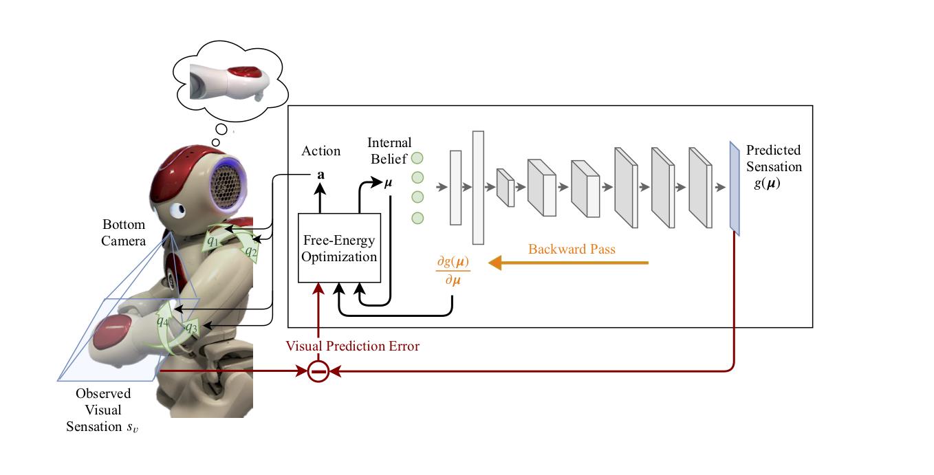
Now that we know more about the FEP we are ready to formalize the body perception and action problem. We developed the first Active Inference model working in a humanoid robot.

Active inference in a humanoid robot and the iCub robot description for the reaching task

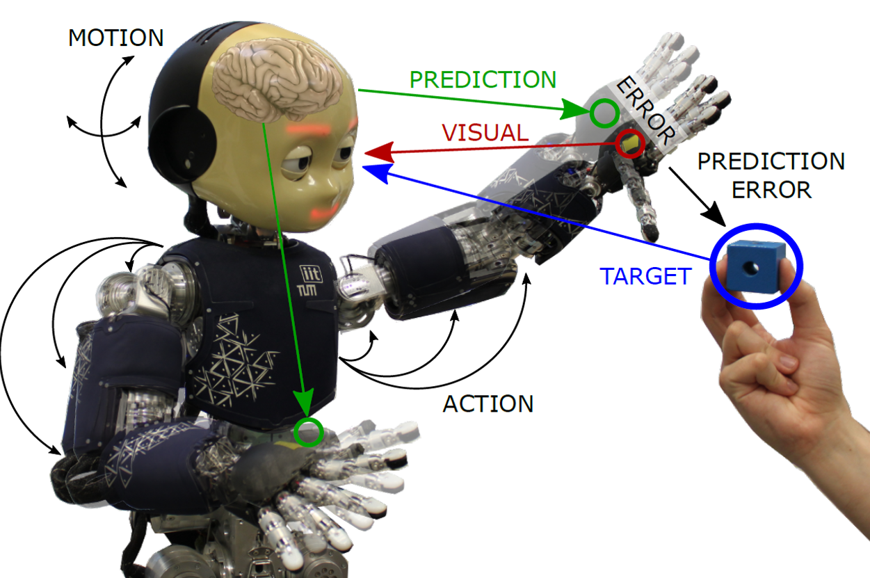
The robot infers its body (e.g., joint angles) by minimizing the prediction error: discrepancy between the sensors (visual and joint) and their expected values. In the presence of error, it changes the perception of its body and generates an action to reduce this discrepancy. Both are computed by optimizing the free-energy bound. Two different tasks are defined: a reaching and a tracking task. First, the object is a causal variable that acts as a perceptual attractor $\rho$, producing an error in the desired sensory state and promoting a reaching action towards the goal. The equilibrium point appears when the hand reaches the object. Meanwhile, the robot’s head keeps the object in its visual field, improving the reaching performance.

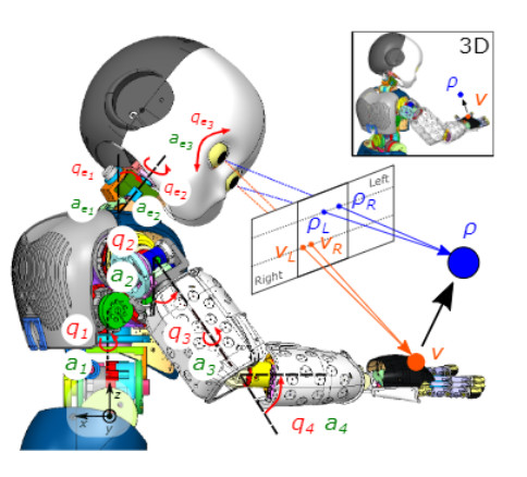
Following the equation development of the previous sections, we will define the Laplace-encoded energy of the system as the product of the likelihood, which accounts for proprioception functions in terms of the current body configuration, and the prior, which includes the dynamic model of the system defining the change of its internal state over time.

Body configuration, or internal variables, is defined as the joint angles. The estimated states $\mu$ are the belief the agent has about the joint angle position and the action $a$ is the angular velocity of those same joints. Due to the fact that we use a velocity control for the joints, first-order dynamics must also be considered $\mu^\prime$

Sensory data will be obtained through several input sensors that provide information about the position of the end-effector in the visual field $s_v$, and joint angle position $s_p$. The dynamic model for the latent variables (joint angles) is determined by a function which depends on both the current state $\mu$ and the causal variables $\rho$ (e.g. 3D position of the object to be reached), with a noisy input following a normal distribution with mean at the value of this function$f(\mu, \rho)$. The reaching goal is defined in the dynamics of the model by introducing a perceptual attractor.

$$p(s, \mu, \rho)=p(s | \mu) p(\mu)=p\left(s_{p} | \mu\right) p\left(s_{v} | \mu\right) p\left(\mu^{\prime} | \mu, \rho\right)$$

Sensory data and dynamic models are assumed to be noisy following a normal distribution, allowing us to define their likelihood functions.

$$\begin{aligned} &p\left(s_{p} | \mu\right)=\mathcal{N}\left(\mu, \Sigma_{s_{p}}\right)\\ &p\left(s_{v} | \mu\right)=\mathcal{N}\left(g(\mu), \Sigma_{s_v}\right)\\ &p\left(\mu^{\prime} | \mu, \rho\right)=\mathcal{N}\left(f(\mu, \rho), \Sigma_{\mu}\right) \end{aligned}$$

Where $g$ is the predictor or forward model of the visual sensation and $f$ is the dynamics of the latent space.

With the variational free-energy of the system defined, we can proceed to its optimization using gradient descent. The differential equations used to update $\mu, \mu^\prime$ and $a$ are:

$$\dot{\mu}=\mu^{\prime}-\frac{\partial F}{\partial \mu} \quad \dot{\mu}^{\prime}=-\frac{\partial F}{\partial \mu^{\prime}} \quad \dot{a}=-\frac{\partial F}{\partial a}$$

And the partial derivatives of the free energy are:

$$\begin{aligned} &-\frac{\partial F}{\partial \mu}=\frac{1}{\Sigma_{s_{p}}}\left(s_{p}-\mu\right)+\frac{1}{\Sigma_{s_{w}}} \frac{\partial g_{v}(\mu)^{T}}{\partial \mu}\left(s_{v}-g(\mu)\right)\\ &\hspace{4em} +\frac{1}{\Sigma_{s_{p}}} \frac{\partial f(\mu, \rho)^{T}}{\partial \mu}\left(\mu^{\prime}-f(\mu, \rho)\right)\\ &-\frac{\partial F}{\partial a}=-\left(\frac{1}{\Sigma_{s_{p}}} \frac{\partial s_{p}}{\partial a}\left(s_{p}-\mu\right)+\frac{1}{\Sigma_{s_{v}}} \frac{\partial s_{v}^{T}}{\partial a}\left(s_{v}-g_{v}(\mu)\right)\right)\\ &-\frac{\partial F}{\partial \mu^{\prime}}=-\frac{1}{\Sigma_{s_{\mu}}}\left(\mu^{\prime}-f(\mu, \rho)\right)=\frac{1}{\Sigma_{s_{\mu}}}\left(f(\mu, \rho)-\mu^{\prime}\right) \end{aligned}$$

Note that all the terms in the update equations have a similar form to:

$$-\underbrace{\frac{\partial g(\mu)^{T}}{\partial \mu}}_{\text {mapping }} \underbrace{\sum_{s}^{-1}}_{\text {precision}} \underbrace{(s-g(\mu))}_{\text {prediction error}}$$

Results

Experiment: Adaptation The robot adapts its reaching behavior when we change the visual feature location that defines the end-effector. A simile would be that we change the length or location of your hand. The optimization process will find an equilibrium between the internal model and the real observation by perceptual updating but also by exerting an action.

Experiment: Comparison Motion from the active inference algorithm is compared to inverse kinematics.

Experiment: Dynamics for 2D and 3D reaching task Body perception and action variables are analyzed during an arm reaching with active head towards a moving object. The head and the eyes are tracking the object in the middle of the image and the arm is performing the reaching task.

More Info

If you are interested in this research and want to learn more, check out the selfception project webpage and the related papers below. We will release the code in open source very soon. The students Guillermo Oliver and Cansu Sancaktar contributed with the research and this blog entry. A full video with all experiments can be watched here.

Check our continuation post Part II to dig into a deep learning version of this approach.

@article{oliver2019active,
  title={Active inference body perception and action for humanoid robots},
  author={Oliver, Guillermo and Lanillos, Pablo and Cheng, Gordon},
  journal={arXiv preprint arXiv:1906.03022},
  year={2019}
}

@inproceedings{lanillos2018adaptive,
  title={Adaptive robot body learning and estimation through predictive coding},
  author={Lanillos, Pablo and Cheng, Gordon},
  booktitle={2018 IEEE/RSJ International Conference on Intelligent Robots and Systems (IROS)},
  pages={4083--4090},
  year={2018},
  organization={IEEE}
}

Acknowledgements. This work has been supported by SELFCEPTION project, European Union Horizon 2020 Programme under grant agreement n. 741941, the European Union’s Erasmus+ Programme, the Institute for Cognitive Systems at the Technical University of Munich (TUM) and the Artificial Cognitive Systems at the Donders Institute for Brain, Cognition and Behaviour.